🐍 Practice n°4: classification
The objective of this session is to learn about classification task. You will have to build a new model only using the text review.
In order to apply classification models, we need to change the target definition. We will divide the reviews into good or bad using the rating.
So our goal is to have a model, a function, that takes text as input and output a label/class (good review or bad review).
$$f(text) = label$$
The data are the same as those used for the regression (source ratebeer dataset description).
Here are the main steps of the notebook :
- What is classification ?
- Focus on logistic regression
- Preparation
- Binary target definition
- Text cleaning
- Modelling
- 6.1 First model using CountVectorizer
- 6.2 Choose the right metrics
- 6.3 Second model using TF-IDF
1. What is classification ?
Classification in machine learning consists of mathematical methods that allow to predict a discrete outcome (y) based on the value of one or more predictor variables (x).
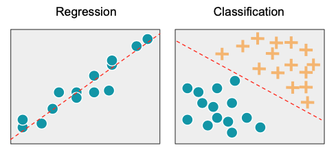
There are several types of classification :
- Binary classification: the task of classifying the data into two groups (each called class).
Example: an email can be classified as belonging to one of two classes: "spam" and "not spam".
- Multi-class classification: the task of classifying the data into N groups (N > 2).
Example: an image can be classified as belonging to one of N classes: "cat", "dog", "cow" or "fish".
- Multi-label classification: this is a generalization of multi-class classification problem where an instance can be assigned to multiple classes.
Example: a movie can be classified as belonging to one or more classes: "action", "adventure", "thriller" or all simultaneously.
In this session, we will focus on the Binary classification.
2. Focus on logistic regression
As seen in the last session, we can represent the link between the explicatives variables and the target to be predicted as follows
$$\hat{y} = \beta_0 + \beta_1x_1 + \beta_2x_2 + ... + \beta_nx_n$$
The difference here is that the target is not a continous variable (rating) but a discrete one (good review / bad review). If we limit ourselves to this model, the linear combination of each input will give an unbounded number that does not allow us to classify the review into good or bad.
To transform the number provided by the linear combination into a classification, we
use a function called sigmoid function which has the interesting property of
transforming the numbers passed inside into numbers between 0 and 1.
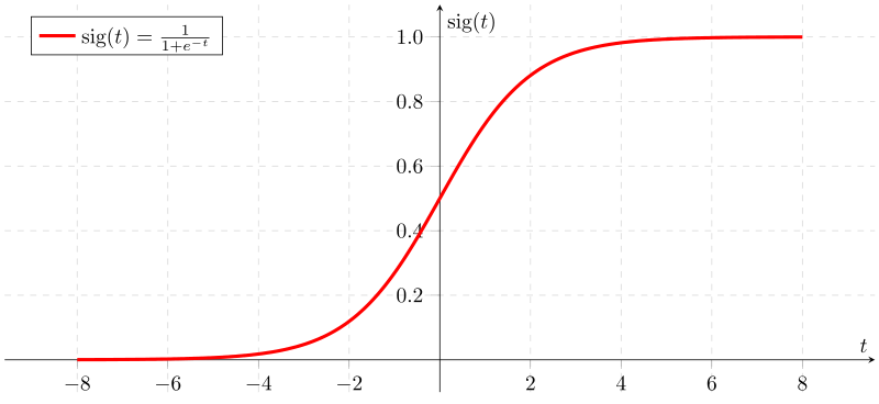
After passing the linear combination through this function, the output will be considered as a probability $P$ and using a threshold (0.5 in general), the review can be classified as bad review, if $P < 0.5$, or good review, if $P >= 0.5$.
This threshold can be modified in some contexts
Then during the training phase, we will compute the parameters β in order to optimize
the Maximum Likelihood i.e., for a given bad review, we want the probalility
estimated by our model to be minimal and for a given good review, we want the
probalility estimated by our model to be maximal.
3. Preparation
Install & import modules
import pandas as pd
import numpy as np
from sklearn.feature_extraction.text import CountVectorizer
from sklearn.feature_extraction.text import TfidfVectorizer
from sklearn.model_selection import train_test_split
from sklearn.linear_model import LogisticRegression
from sklearn.pipeline import Pipeline
from sklearn.metrics import confusion_matrix, accuracy_score, f1_score, recall_score, precision_score, classification_report
import nltk
from nltk.corpus import stopwords
import seaborn as sns
nltk.download('stopwords')

pd.set_option('display.max_colwidth', None)
pd.set_option("display.precision", 2)
sns.set_style("whitegrid")
[nltk_data] Downloading package stopwords to /home/runner/nltk_data...
[nltk_data]   Unzipping corpora/stopwords.zip.
Read remote dataset
file_url = "https://github.com/ML-boot-camp/ratebeer/raw/master/data/ratebeer_sample_enriched.parquet"
df_full = pd.read_parquet(file_url)
df_full.head(5)
| beer | brewery | alcohol | type | rating_appearance | rating_aroma | rating_palate | rating_taste | rating | timestamp | user | text | beer_degree | brewery_degree | user_degree | text_length | date | is_good | |
|---|---|---|---|---|---|---|---|---|---|---|---|---|---|---|---|---|---|---|
| 0 | Breckenridge Oatmeal Stout | 383 | 4.95 | Stout | 4 | 7 | 4 | 7 | 14 | 1217462400 | blutt59 | bottle, oat nose with black color, bitter chocolate flavor with a good coffee cocoa finish | 51 | 413 | 300 | 90 | 2008-07-31 02:00:00 | 0 |
| 1 | Breckenridge 471 Small Batch Imperial Porter | 383 | 7.50 | Imperial/Strong Porter | 3 | 8 | 3 | 8 | 14 | 1312588800 | blutt59 | bottle, received in trade, dark brown with garnet highlights, short lived foam, aroma is quite port like and raisin, flavor is sweet raisin or prune, toasty almond, waffle batter, nice finish | 4 | 413 | 300 | 191 | 2011-08-06 02:00:00 | 0 |
| 2 | Breckenridge Avalanche Amber | 383 | 5.41 | Amber Ale | 3 | 5 | 3 | 5 | 10 | 1205020800 | blutt59 | 12 oz. bottle, amber color with soapy head, slight caramel flavor but watery not much hops some effervescence | 43 | 413 | 300 | 109 | 2008-03-09 01:00:00 | 0 |
| 3 | Breckenridge Lucky U IPA | 383 | 6.20 | India Pale Ale (IPA) | 3 | 6 | 3 | 7 | 12 | 1255737600 | blutt59 | bottle, golden orange color with light tan foam , citric soour aroma with hoppy citrus and lime bitter flavor, could use a little more malt for balance | 20 | 413 | 300 | 151 | 2009-10-17 02:00:00 | 0 |
| 4 | Fullers Vintage Ale 2009 | 55 | 8.50 | English Strong Ale | 3 | 7 | 3 | 8 | 14 | 1282003200 | blutt59 | bottle, thanks to SS, almond amber colored pour with off white soapy foam, fruity metallic aroma, flavors of dried apricots, metallics, fruity medicinal finish | 18 | 978 | 300 | 159 | 2010-08-17 02:00:00 | 0 |
4. Binary target definition
Filter the data using only 1000 reviews and then explore some reviews
# Filter the data
N_rows = 1000
df = df_full[["text", "rating", "is_good"]].sample(N_rows, random_state=42)
# Display some text reviews

print("GUESS THE RATING ?")
df_example = df.sample(n=1)
df_example.text
GUESS THE RATING ?
117167    Cask at Spoons, Milton Keynes. Dark amber with a thick white head. Couldnt pick up an aroma. Faint malty taste overlaid by hops. Oily, creamy mouthfeel, probably thanks to the head, which was courtesy of Mr Wetherspoon. Slight bitter finish. Something lacking here.
Name: text, dtype: object
print(f"RATING: {df_example.rating.iloc[0]}")
RATING: 10
To begin with a binary classification problem, we will bin the target into 2 classes: bad review and good review
First, look at the target distribution and choose a threshlold to identify good reviews from the rest.
# display the target distribution
df.rating.astype(int).plot(kind="hist")
<Axes: ylabel='Frequency'>

You can play with the rating_threshold and look at the new target distribution.
# Create a binary target and display the target distribution
rating_threshold = 16 # LINE TO BE REMOVED FOR STUDENTS
(df.rating >= rating_threshold).astype(int).value_counts(normalize=True)
rating
0    0.74
1    0.26
Name: proportion, dtype: float64
Usually the threshold is defined by looking manually at the data: annotating a few
reviews as "good" or "bad" and see which ratings they had.
E.g: on google maps a "good" review is above 4 stars (out of 5 stars).
For simplicity, here we'll use the is_good binary target defined during the data
engineering phase.
# Create a binary target and display the target distribution
rating_threshold = df.rating.median() # LINE TO BE REMOVED FOR STUDENTS
(df.rating >= rating_threshold).astype(int).value_counts(normalize=True)
rating
1    0.56
0    0.44
Name: proportion, dtype: float64
5. Text cleaning
From text reviews to numerical vectors
Before training some models, the first step is to transform text into numbers :
from
f(raw_text) = rating_classe
to
f(numerical_vector_representing_text) = rating_classe
Indeed, we can't direclty feed an algortihm with text.
For example:
Wow, that beer is SOOOO good :O !!
must be transformed to something like:
[3, 4, 21, 0, 0, 8, 19]
where the values of the vector contain the meaning of the text. Knowing that the closer texts are in terms of meaning, the more closed their vector representation is too. Moreover, it is often more convenient to convert texts of different sizes into vectors of fixed size.
For example:
"Wow, that beer is SOOOO good :O !!"
-> characters : 34
-> vector (1x7) : [3, 4, 21, 0, 0, 8, 19]
"This beer is very tasty"
-> characters : 23
-> vector (1x7) : [3, 4, 20, 0, 0, 7, 19]
But:
"It's not a beer, just motor oil at best."
-> characters : 40
-> vector (1x7) : [0, 4, 1, 12, 14, 0, 0]
From raw text reviews to clean list of words
Before converting text to numerical vector, the first step is to clean the text to keep only the pertinent information.
Here are the following cleaning steps that we will apply on the reviews:
- Convert letter to lowercase
"Wow, that beer is SOOOO good :O !!" -> "wow, that beer is soooo good :o !!"
- Remove the punctuation letter to lowercase
"wow, that beer is soooo good :o !!" -> "wow that beer is soooo good"
- Transform the text into tokens
"wow that beer is soooo good" -> ["wow", "that", "beer", "is", "soooo", "good"]
- Remove the stopwords, the most common english words that often bring noise to the models.
["wow", "that", "beer", "is", "soooo", "good"] -> ["wow", "beer", "soooo", "good"]
- To go further, some techniques can be used to reduce the forms of each word into a common base or root. This can be done with:
(1) Stemming is the process of eliminating affixes (suffixed, prefixes, infixes, circumfixes) from a word in order to obtain a word stem.
am, are, is $\Rightarrow$ be
(2) Lemmatization is related to stemming, differing in that lemmatization is able to capture canonical forms based on a word's lemma.
book, books, book's, book' $\Rightarrow$ book
The steps presented here are just the most basic, many different things can be applied to the cleaning part of the text.
def convert_text_to_lowercase(df, colname):
    df[colname] = (
        df[colname]
        .str.lower() # LINE TO BE REMOVED FOR STUDENTS
    )
    return df

def not_regex(pattern):
        return r"((?!{}).)".format(pattern)

def remove_punctuation(df, colname):
    df[colname] = df[colname].str.replace("\n", " ")
    df[colname] = df[colname].str.replace("\r", " ")
    alphanumeric_characters_extended = "(\\b[-/]\\b|[a-zA-Z0-9])"
    df[colname] = df[colname].str.replace(not_regex(alphanumeric_characters_extended), " ")
    return df

def tokenize_sentence(df, colname):
    df[colname] = df[colname].str.split()
    return df

def remove_stop_words(df, colname):
    stop_words = stopwords.words("english")
    df[colname] = df[colname].apply(lambda x: [word for word in x if word not in stop_words])
    return df

def reverse_tokenize_sentence(df, colname):
    df[colname] = df[colname].map(lambda word: " ".join(word))
    return df


def text_cleaning(df, colname):
    """
    Takes in a string of text, then performs the following:
    1. convert text to lowercase
    2. remove punctuation and new line characters "\n"
    3. Tokenize sentences
    4. Remove all stopwords
    5. convert tokenized text to text
    """
    df = (
        df
        .pipe(convert_text_to_lowercase, colname) # LINE TO BE REMOVED FOR STUDENTS
        .pipe(remove_punctuation, colname) # LINE TO BE REMOVED FOR STUDENTS
        .pipe(tokenize_sentence, colname) # LINE TO BE REMOVED FOR STUDENTS
        .pipe(remove_stop_words, colname) # LINE TO BE REMOVED FOR STUDENTS
        .pipe(reverse_tokenize_sentence, colname) # LINE TO BE REMOVED FOR STUDENTS
    )
    return df
# Apply data cleaning
df_cleaned = text_cleaning(
    df, # LINE TO BE REMOVED FOR STUDENTS
    "text"
)
# Control the cleaning
df_cleaned.head()
| text | rating | is_good | |
|---|---|---|---|
| 119737 | 0.33l 2009-bottle. pours deep red body thin bubbly side-sticking almost yellow-beige head. aroma lovely caramel sweet, hops, smoke brown sugar. medium-bodied medium+ carbonated. quite boozy first, caramel- brown sugar-sweet slight floral note. something barlywines normally sweet me, sweet, sweet first would thought. also strong bitterness equalized sweetness. combined warming alcohol made pleasant experience. | 15 | 0 |
| 72272 | another nice seasonal muskoka. pours nice dark brown beige frothy head goes nice covering top. nose lotsa chocolate cocoa. mouth feel touch thin otherwise works well. flavor lotsa chocolate touch cranberries decent well hidden amount booze. | 16 | 1 |
| 158154 | pours hazy, white hued light golden, aroma sweet, estery fruity notes banana sweet melon prevalent. rich chewy mouth anise-like bitterness nice light burn finish, slightly warming. | 14 | 0 |
| 65426 | served draft beer run charlottesville, va 3/30/11. pours clear copper color medium sized creamy tan head. good head retention lacing. aroma pretty much straight bourbon toffee notes quite bit booze. taste bourbon, vanilla, toffee, caramel, booze lightly toasty finish. medium bodied. | 15 | 0 |
| 30074 | tap old hat. listed "amber rhy" scoreboard inclined think spelling error brewpub staff. cloudy orange-red body, thin light cream head. sweet grainy aroma notes caramel. flavor caramely, fruity sweetness stout doppelbock had, beer boring comparison. little rye character permeated unrefined sweetness. sharp carbonation, bland beer. something uninitiated, suppose. | 12 | 0 |
We still have to transform the list of tokens to a fixed size numerical vector
For that, we will use 2 very common techniques : CountVectorizer and TF-IDF
1) CountVectorizer:
CountVectorizer is used to convert a collection of text documents to a vector of token counts.
Example:
["beer", "most", "tasty", "beer", "world"]
Will be transformed into ⬇
| beer | most | tasty | world |
|---|---|---|---|
| 2 | 1 | 1 | 1 |
In practice, you have to define a vocabulary size and each text will be transform into a vector of size [1 x vocabulary size]. Consequently, zeros will be added to the vector for each word present in the corpus vocabulary but missing in the specific review. The vocabulary space is defined using term frequency across the corpus: the most frequent words are kept.
2) TF-IDF (optional):
TF-IDF or term frequency–inverse document frequency, is a numerical statistic that is intended to reflect how important a word is to reflect how important a word is to a document in a collection or corpus.
TF: Term Frequency, which measures how frequently a term occurs in a document. Since every document is different in length, it is possible that a term would appear much more times in long documents than shorter ones. Thus, the term frequency is often divided by the document length (aka. the total number of terms in the document) as a way of normalization:
TF(t) = (Nbr of times term t appears in a document) / (Total nbr of terms in the
document)
IDF: Inverse Document Frequency, which measures how important a term is. While computing TF, all terms are considered equally important. However it is known that certain terms, such as "is", "of", and "that", may appear a lot of times but have little importance. Thus we need to weigh down the frequent terms while scale up the rare ones, by computing the following:
IDF(t) = log(Total number of documents / Number of documents with term t in it)
Example:
Consider a document containing 100 words wherein the word book appears 3 times. The term frequency (i.e., tf) for cat is:
TF(t) = (Nbr of times term t appears in a document) / (Total nbr of terms in the
document)
      = 3 / 100
      = 0.03
Now, assume we have 10 million documents and the word book appears in one thousand of these. Then, the inverse document frequency (i.e., idf) is calculated as
IDF(t) = log(Total number of documents / Number of documents with term t in it)
       = log(10,000,000 / 1,000)
       = 4
Thus, the Tf-idf weight is the product of these quantities:
Tf-IDF = TF(t) * IDF(t)
       = 0.03 * 4
       = 0.12
Split the data into train/test sets
Before applying these transormation on the text, we will just split the data for the modelling part.
Keep 20% of the data for the test dataset
TARGET = "is_good" # LINE TO BE REMOVED FOR STUDENTS
FEATURE = "text" # LINE TO BE REMOVED FOR STUDENTS

x_train, x_test, y_train, y_test = train_test_split(
    df_cleaned[FEATURE], # LINE TO BE REMOVED FOR STUDENTS
    df_cleaned[TARGET], # LINE TO BE REMOVED FOR STUDENTS
    test_size=0.2,
    random_state=42)
6. Modelling
6.1 First model using CountVectorizer
Transform the text reviews into numerical vectors by counting the number of words in each reviews. Use the scikit-learn library.
In order not to bring information from the train set into the test set, you must train the CountVectorizer on the train set and apply it to the test set.
Hint:
# Define the vocabulary size to 100
count_vectorizer = CountVectorizer(
    analyzer="word",
    max_features=100 # LINE TO BE REMOVED FOR STUDENTS
    )
# Apply the CountVectorizer and check the results on some rows
count_vectorizer.fit(x_train)

x_train_features = count_vectorizer.transform(x_train).toarray()
x_test_features = count_vectorizer.transform(x_test).toarray()
x_train_features[0]
array([0, 0, 0, 0, 0, 0, 0, 0, 0, 0, 0, 0, 0, 0, 0, 1, 0, 1, 0, 0, 0, 0,
       0, 0, 0, 0, 0, 0, 1, 0, 0, 0, 0, 0, 0, 0, 0, 0, 0, 0, 0, 0, 0, 0,
       1, 0, 0, 0, 0, 0, 0, 1, 3, 0, 0, 0, 0, 0, 0, 0, 0, 0, 1, 0, 0, 0,
       0, 0, 0, 0, 0, 0, 0, 0, 0, 0, 0, 0, 0, 0, 0, 0, 0, 1, 0, 0, 0, 0,
       0, 0, 0, 0, 1, 0, 0, 0, 0, 0, 0, 0])
x_train.iloc[0]
'bottle home ... colins tasting ... deep hazy brown ... thin lacing ... light sour cheery light strawb nose ... tart sourness ... cherry ... light sourness ... ok.'
The next step is to define the model that will use in input the vectors from the the
CountVectorizer. We will use a logistic regression model, using again the
scikit-learn library.
In order to produce cleaner code, we can combine these 2 steps (CountVectorizer and Logistic regression) into a single pipeline.
- Initialize the
CountVectorizer - Initialize the
LogisticRegression - Define your
Pipelineobject with these 2 steps - Fit the
Pipeline
Hint:
# Initialize the CountVectorizer
count_vectorizer = CountVectorizer(
    analyzer="word",
    max_features=100
    )

# Initialize the logistic regression
logit = LogisticRegression(solver="lbfgs", verbose=2, n_jobs=-1)

# Combine them into a Pipeline object
pipeline_cv = Pipeline([
    ("vectorizer", count_vectorizer), # LINE TO BE REMOVED FOR STUDENTS
    ("model", logit)]) # LINE TO BE REMOVED FOR STUDENTS

# Fit the Pipeline
pipeline_cv.fit(x_train, y_train)
[Parallel(n_jobs=-1)]: Using backend LokyBackend with 2 concurrent workers.
RUNNING THE L-BFGS-B CODE

           * * *

Machine precision = 2.220D-16
 N =          101     M =           10

At X0         0 variables are exactly at the bounds

At iterate    0    f=  5.54518D+02    |proj g|=  2.04000D+02

At iterate    1    f=  5.31344D+02    |proj g|=  8.78928D+01

At iterate    2    f=  4.55160D+02    |proj g|=  4.01187D+01

At iterate    3    f=  4.32123D+02    |proj g|=  8.26324D+01

At iterate    4    f=  4.16715D+02    |proj g|=  3.98241D+01

At iterate    5    f=  3.97087D+02    |proj g|=  1.47372D+01

At iterate    6    f=  3.65120D+02    |proj g|=  1.53607D+01

At iterate    7    f=  3.40922D+02    |proj g|=  1.62430D+01

At iterate    8    f=  3.29177D+02    |proj g|=  3.47076D+00

At iterate    9    f=  3.27222D+02    |proj g|=  3.63787D+00

At iterate   10    f=  3.24542D+02    |proj g|=  4.96374D+00

At iterate   11    f=  3.22516D+02    |proj g|=  3.37517D+00

At iterate   12    f=  3.21303D+02    |proj g|=  1.66355D+00

At iterate   13    f=  3.21030D+02    |proj g|=  1.21264D+00

At iterate   14    f=  3.20910D+02    |proj g|=  4.79720D-01

At iterate   15    f=  3.20867D+02    |proj g|=  2.75051D+00

At iterate   16    f=  3.20817D+02    |proj g|=  7.42277D-01

At iterate   17    f=  3.20805D+02    |proj g|=  3.80123D-01

At iterate   18    f=  3.20798D+02    |proj g|=  2.03584D-01

At iterate   19    f=  3.20788D+02    |proj g|=  1.89959D-01

At iterate   20    f=  3.20780D+02    |proj g|=  1.59201D-01

At iterate   21    f=  3.20776D+02    |proj g|=  1.64005D-01

At iterate   22    f=  3.20775D+02    |proj g|=  6.25600D-02

At iterate   23    f=  3.20774D+02    |proj g|=  3.73012D-02

At iterate   24    f=  3.20774D+02    |proj g|=  2.13423D-02

At iterate   25    f=  3.20774D+02    |proj g|=  3.09411D-02

At iterate   26    f=  3.20774D+02    |proj g|=  1.86634D-02

At iterate   27    f=  3.20774D+02    |proj g|=  1.77506D-02

At iterate   28    f=  3.20774D+02    |proj g|=  1.19104D-02

At iterate   29    f=  3.20774D+02    |proj g|=  6.78925D-03

At iterate   30    f=  3.20774D+02    |proj g|=  4.54960D-03

At iterate   31    f=  3.20774D+02    |proj g|=  4.83343D-03

At iterate   32    f=  3.20774D+02    |proj g|=  8.18759D-03

           * * *

Tit   = total number of iterations
Tnf   = total number of function evaluations
Tnint = total number of segments explored during Cauchy searches
Skip  = number of BFGS updates skipped
Nact  = number of active bounds at final generalized Cauchy point
Projg = norm of the final projected gradient
F     = final function value

           * * *

   N    Tit     Tnf  Tnint  Skip  Nact     Projg        F
  101     32     35      1     0     0   8.188D-03   3.208D+02
  F =   320.77383276003553

CONVERGENCE: REL_REDUCTION_OF_F_<=_FACTR*EPSMCH
This problem is unconstrained.
Pipeline(steps=[('vectorizer', CountVectorizer(max_features=100)),
                ('model', LogisticRegression(n_jobs=-1, verbose=2))])
In a Jupyter environment, please rerun this cell to show the HTML representation or trust the notebook. On GitHub, the HTML representation is unable to render, please try loading this page with nbviewer.org.
Pipeline(steps=[('vectorizer', CountVectorizer(max_features=100)),
('model', LogisticRegression(n_jobs=-1, verbose=2))])CountVectorizer(max_features=100)
LogisticRegression(n_jobs=-1, verbose=2)
Now you can make predictions on the test set
# predictions
y_pred_cv = pipeline_cv.predict(x_test)
How to evaluate our model ?
Accuracy is the most intuitive performance measure and it is simply a ratio of
correctly predicted observation to the total observations
# Compute accuracy
print(f"model accuracy : {accuracy_score(y_pred_cv, y_test)} %")
model accuracy : 0.72 %
What is you opinion about the accuracy score ?
One may think that, if we have high accuracy then our model is best. Yes, accuracy is a great measure but only when you have symmetric datasets where values of false positive and false negatives are almost same. Therefore, you have to look at other parameters to evaluate the performance of your model.
One might think that if we have high accuracy, our model is the best. Yes, accuracy is an excellent measure, but only when you have balanced data (i.e. an equivalent representation of each class in the data).
Let's do a test with a reference model to show how accuracy can be a source of error when evaluating a model: Create a model that predict everytime the most frequent class and compare the results.
# Baseline model: predict the most-frequent class
y_pred_baseline = [y_test.mode()[0]] * len(y_test)

# Compute accuracy
print(f"model baseline accuracy : {accuracy_score(y_pred_baseline, y_test)} %")
model baseline accuracy : 0.7 %
Accuracy are closed, but the last model is completely idiot !
In case of an imbalanced target (let's say 99% zeros), the accuracy of this dumb model will be 99% !
Therefore, you need to look at other metrics to evaluate the performance of your model.
6.2 Choose the right metrics
We need now define other metrics to evaluate our model.
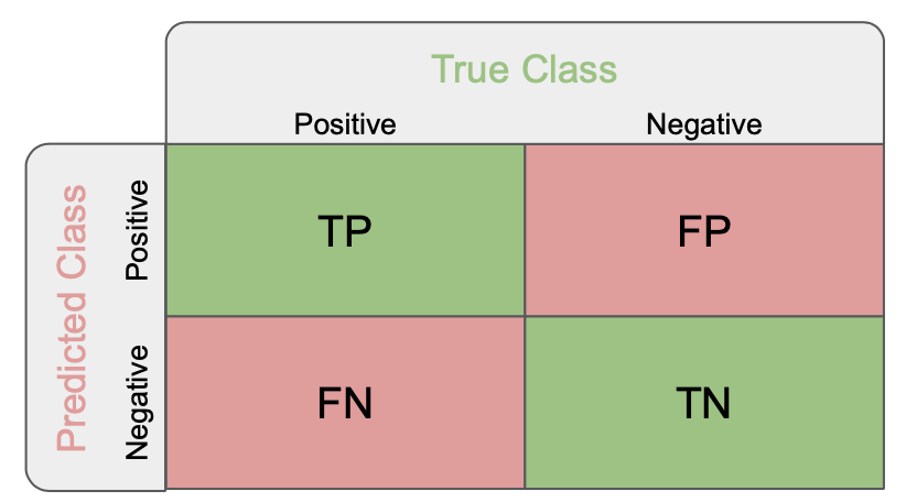
True Positives (TP): these are the correctly predicted positive values which means that the value of actual class is yes and the value of predicted class is also yes.
True Negatives (TN): these are the correctly predicted negative values which means that the value of actual class is no and value of predicted class is also no.
False Positives (FP): when actual class is no and predicted class is yes.
False Negatives (FN): when actual class is yes but predicted class in no.
Accuracy: the ratio of correctly predicted observation to the total observations.
Accuracy = $\frac{TP+TN}{TP+FP+FN+TN}$
- Precision: Precision is the ratio of correctly predicted positive observations to the total predicted positive observations. High precision relates to the low false positive rate.
Precision = $\frac{TP}{TP+FP}$
- Recall (Sensitivity): Recall is the ratio of correctly predicted positive observations to the all observations in actual class - yes.
Recall = $\frac{TP}{TP+FN}$
- F1 score: F1 Score is the weighted average of Precision and Recall. Therefore, this score takes both false positives and false negatives into account. Intuitively it is not as easy to understand as accuracy, but F1 is usually more useful than accuracy, especially if you have an uneven class distribution.
F1 Score = $2* \frac{Recall * Precision}{Recall + Precision}$
Let's now compare again our 2 models !
First, plot the confusion matrix, the precision, recall and f1 score for each model. You can also print the classification report of scikit learn that sums up the main classification metrics.
Hint:
# Confusion matrices
print(f"Confusion matrix of the first model: \n {confusion_matrix(y_test, y_pred_cv)}")
print(f"Confusion matrix of the baseline model: \n {confusion_matrix(y_test, y_pred_baseline)}")
Confusion matrix of the first model:
 [[122  18]
 [ 38  22]]
Confusion matrix of the baseline model:
 [[140   0]
 [ 60   0]]
# Evaluate the first model
print(f"first model precision : {precision_score(y_pred_cv, y_test):.{3}f}%")
print(f"first model recall    : {recall_score(y_pred_cv, y_test)}%")
print(f"first model f1 score  : {f1_score(y_pred_cv, y_test):.{3}f}%\n")

# Evaluate the baseline model
print(f"baseline model precision : {precision_score(y_pred_baseline, y_test)}%")
print(f"baseline model recall    : {recall_score(y_pred_baseline, y_test)}%")
print(f"baseline model f1 score  : {f1_score(y_pred_baseline, y_test)}%")
first model precision : 0.367%
first model recall    : 0.55%
first model f1 score  : 0.440%

baseline model precision : 0.0%
baseline model recall    : 0.0%
baseline model f1 score  : 0.0%
/home/runner/micromamba/envs/ml-bootcamp/lib/python3.11/site-packages/sklearn/metrics/_classification.py:1469: UndefinedMetricWarning: Recall is ill-defined and being set to 0.0 due to no true samples. Use `zero_division` parameter to control this behavior.
  _warn_prf(average, modifier, msg_start, len(result))
# Classification report
print(classification_report(
    y_test, y_pred_cv # LINE TO BE REMOVED FOR STUDENTS
))
              precision    recall  f1-score   support

           0       0.76      0.87      0.81       140
           1       0.55      0.37      0.44        60

    accuracy                           0.72       200
   macro avg       0.66      0.62      0.63       200
weighted avg       0.70      0.72      0.70       200
# Classification report
print(classification_report(y_test, y_pred_baseline))
              precision    recall  f1-score   support

           0       0.70      1.00      0.82       140
           1       0.00      0.00      0.00        60

    accuracy                           0.70       200
   macro avg       0.35      0.50      0.41       200
weighted avg       0.49      0.70      0.58       200
/home/runner/micromamba/envs/ml-bootcamp/lib/python3.11/site-packages/sklearn/metrics/_classification.py:1469: UndefinedMetricWarning: Precision and F-score are ill-defined and being set to 0.0 in labels with no predicted samples. Use `zero_division` parameter to control this behavior.
  _warn_prf(average, modifier, msg_start, len(result))
6.3 Second model using TF-IDF Vectorizer (optional)
In this last section, you will use a better approach in term of vectorization: TF-IDF
Scikit-learn provide the TfidfVectorizer that can be used in the same way as
CountVectorizer.
Hint:
# Initialize the TF-IDF
tfidf_vectorizer = TfidfVectorizer(
    analyzer='word',
    max_features=100 # LINE TO BE REMOVED FOR STUDENTS
    )

# Apply the TfidfVectorizer and check the results on some rows
tfidf_vectorizer.fit(x_train)

x_train_features = tfidf_vectorizer.transform(x_train).toarray()
x_test_features = tfidf_vectorizer.transform(x_test).toarray()
x_train_features[0]
array([0.        , 0.        , 0.        , 0.        , 0.        ,
       0.        , 0.        , 0.        , 0.        , 0.        ,
       0.        , 0.        , 0.        , 0.        , 0.        ,
       0.19400832, 0.        , 0.22794963, 0.        , 0.        ,
       0.        , 0.        , 0.        , 0.        , 0.        ,
       0.        , 0.        , 0.        , 0.32713051, 0.        ,
       0.        , 0.        , 0.        , 0.        , 0.        ,
       0.        , 0.        , 0.        , 0.        , 0.        ,
       0.        , 0.        , 0.        , 0.        , 0.30997343,
       0.        , 0.        , 0.        , 0.        , 0.        ,
       0.        , 0.28915725, 0.59635253, 0.        , 0.        ,
       0.        , 0.        , 0.        , 0.        , 0.        ,
       0.        , 0.        , 0.26488472, 0.        , 0.        ,
       0.        , 0.        , 0.        , 0.        , 0.        ,
       0.        , 0.        , 0.        , 0.        , 0.        ,
       0.        , 0.        , 0.        , 0.        , 0.        ,
       0.        , 0.        , 0.        , 0.34835863, 0.        ,
       0.        , 0.        , 0.        , 0.        , 0.        ,
       0.        , 0.        , 0.27665128, 0.        , 0.        ,
       0.        , 0.        , 0.        , 0.        , 0.        ])
x_train.iloc[0]
'bottle home ... colins tasting ... deep hazy brown ... thin lacing ... light sour cheery light strawb nose ... tart sourness ... cherry ... light sourness ... ok.'
You can now combine the vectorizer to a logistic regression in a single pipeline
# Initialize the TfidfVectorizer
tfidf_vectorizer = TfidfVectorizer(
    analyzer='word',
    max_features=100
    )

# Initialize the logistic regression
logit = LogisticRegression(solver='lbfgs', verbose=2, n_jobs=-1)

# Combine them into a Pipeline object
pipeline_tfidf = Pipeline([
    ('vectorizer', tfidf_vectorizer), # LINE TO BE REMOVED FOR STUDENTS
    ('model', logit)]) # LINE TO BE REMOVED FOR STUDENTS

# Fit the Pipeline
pipeline_tfidf.fit(x_train, y_train)
[Parallel(n_jobs=-1)]: Using backend LokyBackend with 2 concurrent workers.
RUNNING THE L-BFGS-B CODE

           * * *

Machine precision = 2.220D-16
 N =          101     M =           10

At X0         0 variables are exactly at the bounds

At iterate    0    f=  5.54518D+02    |proj g|=  2.04000D+02

At iterate    1    f=  4.43986D+02    |proj g|=  9.94050D+00

At iterate    2    f=  4.41607D+02    |proj g|=  5.63999D+00

At iterate    3    f=  4.31240D+02    |proj g|=  2.62300D+01

At iterate    4    f=  4.16711D+02    |proj g|=  4.32906D+01

At iterate    5    f=  3.94456D+02    |proj g|=  4.20929D+01

At iterate    6    f=  3.76615D+02    |proj g|=  8.35456D+00

At iterate    7    f=  3.75845D+02    |proj g|=  1.10314D+00

At iterate    8    f=  3.75745D+02    |proj g|=  2.13981D+00

At iterate    9    f=  3.75463D+02    |proj g|=  2.69875D+00

At iterate   10    f=  3.74909D+02    |proj g|=  1.97574D+00

At iterate   11    f=  3.74747D+02    |proj g|=  2.81994D-01

At iterate   12    f=  3.74739D+02    |proj g|=  9.21477D-02

At iterate   13    f=  3.74736D+02    |proj g|=  1.40607D-01

At iterate   14    f=  3.74733D+02    |proj g|=  3.94355D-01

At iterate   15    f=  3.74732D+02    |proj g|=  9.60931D-02

At iterate   16    f=  3.74731D+02    |proj g|=  1.79723D-02

At iterate   17    f=  3.74731D+02    |proj g|=  2.14785D-02

At iterate   18    f=  3.74731D+02    |proj g|=  1.95197D-02

At iterate   19    f=  3.74731D+02    |proj g|=  6.76658D-02

At iterate   20    f=  3.74731D+02    |proj g|=  3.09067D-02

At iterate   21    f=  3.74731D+02    |proj g|=  7.79600D-03

At iterate   22    f=  3.74731D+02    |proj g|=  5.07095D-03

At iterate   23    f=  3.74731D+02    |proj g|=  6.33766D-03

At iterate   24    f=  3.74731D+02    |proj g|=  2.25929D-03

At iterate   25    f=  3.74731D+02    |proj g|=  1.51012D-03

At iterate   26    f=  3.74731D+02    |proj g|=  1.39964D-03

           * * *

Tit   = total number of iterations
Tnf   = total number of function evaluations
Tnint = total number of segments explored during Cauchy searches
Skip  = number of BFGS updates skipped
Nact  = number of active bounds at final generalized Cauchy point
Projg = norm of the final projected gradient
F     = final function value

           * * *

   N    Tit     Tnf  Tnint  Skip  Nact     Projg        F
  101     26     30      1     0     0   1.400D-03   3.747D+02
  F =   374.73103485123914

CONVERGENCE: REL_REDUCTION_OF_F_<=_FACTR*EPSMCH
This problem is unconstrained.
Pipeline(steps=[('vectorizer', TfidfVectorizer(max_features=100)),
                ('model', LogisticRegression(n_jobs=-1, verbose=2))])
In a Jupyter environment, please rerun this cell to show the HTML representation or trust the notebook. On GitHub, the HTML representation is unable to render, please try loading this page with nbviewer.org.
Pipeline(steps=[('vectorizer', TfidfVectorizer(max_features=100)),
('model', LogisticRegression(n_jobs=-1, verbose=2))])TfidfVectorizer(max_features=100)
LogisticRegression(n_jobs=-1, verbose=2)
# Predictions
y_pred_tfidf = pipeline_tfidf.predict(x_test)

# Evaluate the second model
print(f"Confusion matrix of the first model: \n {confusion_matrix(y_test, y_pred_tfidf)}")
print(f"second model precision : {precision_score(y_pred_tfidf, y_test):.{3}f}%")
print(f"second model recall    : {recall_score(y_pred_tfidf, y_test)}%")
print(f"second model f1 score  : {f1_score(y_pred_tfidf, y_test):.{3}f}%\n")
Confusion matrix of the first model:
 [[138   2]
 [ 49  11]]
second model precision : 0.183%
second model recall    : 0.8461538461538461%
second model f1 score  : 0.301%
# Classification report
print(classification_report(y_test, y_pred_tfidf))
              precision    recall  f1-score   support

           0       0.74      0.99      0.84       140
           1       0.85      0.18      0.30        60

    accuracy                           0.74       200
   macro avg       0.79      0.58      0.57       200
weighted avg       0.77      0.74      0.68       200
6.4 Optimize the model
You can now try to optimize the model by changing a lot of parameters:
- Take more reviews in input
- Increase the
max_featuresparameter - Remove the most frequent words
- Try adding n-grams to the vectorizer
- Improve the text cleaning
- etc...