Basic data engineering
Join, group by & aggregate
Join
Join type
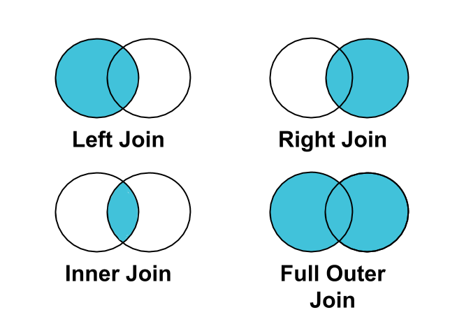
A join is a database operation that combines rows from two tables based on a related column between them, allowing you to query data from both tables as if they were a single entity. Different types of joins determine which rows are included in the result, providing flexibility in how the tables are merged.
| Join type | Description | Includes all data from | May loose data from |
|---|---|---|---|
| Inner | Combines matching rows from both tables | None | Both |
| Left | Includes all rows from the left table | Left | Right |
| Right | Includes all rows from the right table | Right | Left |
| Outer | Combines all rows from both tables, matching where possible | Both | None |
Join types are related to the concepts of inclusion and completeness:
- Use outer join, if you don't want to loose data, but you may have incomplete data.
- Use inner join, if you don't want to have incomplete data, but you may loose data.
Note
When exploring data using pandas, always start your joins
(using the
merge
method) by:
- doing an outer join (
how="outer") - checking the result of the join in the
_mergecolumn (e.g: using thevalue_countsmethod)
E.g:
result = (
    df1
    .merge(df2, on="key_column", how="outer")
    ._merge
    .value_counts()
)
This shows how many rows are coming from each dataframe (both, left_only or
right_only).
Matching type
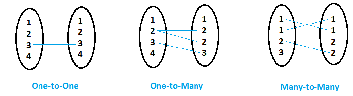
A matching type refers to the relationship between key columns in the tables being joined, such as one-to-one, one-to-many, or many-to-many. It defines how many records in one table correspond to records in another, guiding the structure of the join and affecting the final result.
| Matching Type | Description | Example |
|---|---|---|
| One-to-One (1:1) | Each row in the first table corresponds to one row in the second table. | Employee to Social Security Number |
| One-to-Many (1:m) | Each row in the first table corresponds to multiple rows in the second table. | Customer to Orders (One customer, many orders) |
| Many-to-Many (m:m) | Multiple rows in the first table correspond to multiple rows in the second table. | Products to Categories (Many products, many categories) |
Matching types are related to the concept of cardinality.
In a one-to-one matching:
- The cardinality of the inner join is the cardinality of the intersection \( | L \cap R | \).
- The cardinality of the outer join is the cardinality of the union \( | L \cup R | \).
Whereas one-to-many, many-to-one or many-to-many matchings do duplicate rows in the join result and don't preserve cardinality.
Note
When exploring data using pandas, always use the
validate argument specify the matching type of your joins to avoid unpleasant
surprises. Like:
validate="1:1"validate="1:m"validate="m:1"validate="m:m"(No effect for this one. Can you guess why?)
E.g:
df1.merge(df2, on="key_column", how="inner", validate="1:1")
Key type
Key columns have 2 types:
- Key columns that have unique values are called primary keys. In other words, a primary key uniquely identifies each row within a table.
- Key columns in a table that are referring to a primary key in another table are called foreign keys. In other words, a foreign key links the data from one table to another (but its values are not expected to be unique !).
A join between 2 tables using:
- 2 primary keys is a one-to-one matching
- 1 primary key and 1 foreign key is a one-to-many matching
- 2 foreign keys is a many-to-many matching
Examples
Let's use 2 example tables:
Customers table
| customer_id | name |
|---|---|
| 1 | Alice |
| 2 | Bob |
| 3 | Carol |
Orders table
| order_id | customer_id | total_price |
|---|---|---|
| 101 | 1 | 100 |
| 102 | 2 | 200 |
| 103 | 4 | 150 |
Inner Join on customer_id: combines rows that are matching customer IDs in both
data frames.
| customer_id | name | order_id | total_price |
|---|---|---|---|
| 1 | Alice | 101 | 100 |
| 2 | Bob | 102 | 200 |
Left Join on customer_id: same tables as Inner Join, but includes all customer
rows.
| customer_id | name | order_id | total_price |
|---|---|---|---|
| 1 | Alice | 101 | 100 |
| 2 | Bob | 102 | 200 |
| 3 | Carol | NaN | NaN |
Right Join on customer_id: includes all order rows and matched customer rows.
| customer_id | name | order_id | total_price |
|---|---|---|---|
| 1 | Alice | 101 | 100 |
| 2 | Bob | 102 | 200 |
| NaN | NaN | 103 | 150 |
Outer Join on customer_id: includes all rows from both data frames.
| customer_id | name | order_id | total_price |
|---|---|---|---|
| 1 | Alice | 101 | 100 |
| 2 | Bob | 102 | 200 |
| 3 | Carol | NaN | NaN |
| NaN | NaN | 103 | 150 |
Groupby and aggregation
Group by divides rows into groups based on column values and aggregation operations (like sum, average, or maximum) condense these groups into summary data. This allows for targeted analysis of specific segments of your data.
Aggregation types
Here are the most common SQL aggregation functions:
| SQL Function | Description |
|---|---|
SUM |
Adds up the values in a numeric column |
AVG |
Calculates the average of a numeric column |
COUNT |
Counts the number of rows in a column or table |
MAX |
Returns the maximum value in a column |
MIN |
Returns the minimum value in a column |
MEDIAN |
Finds the middle value of a numeric column |
MODE |
Finds the most frequently occurring value in a column |
STDDEV |
Calculates the standard deviation of a numeric column |
VARIANCE |
Calculates the variance of a numeric column |
FIRST |
Returns the first value in a column (order may vary by DBMS) |
LAST |
Returns the last value in a column (order may vary by DBMS) |
These functions provide various ways to summarize and analyze data. Different databases might offer additional aggregation functions tailored to specific needs or data types.
Note
The behavior of "FIRST" and "LAST" may depend on the database management system (DBMS) and how the data is ordered in the query. In some systems, you may need to use specific ordering clauses to get the desired behavior.
Example
Customer & orders table (join between customers and orders):
| CustomerID | Name | OrderID | Amount |
|---|---|---|---|
| 1 | Alice | 1 | 100 |
| 1 | Alice | 3 | 200 |
| 2 | Bob | 2 | 50 |
| 3 | Charlie | 4 | 150 |
In SQL, if we want to find the total amount spent by each customer, we'll use a
GROUP BY operation on the CustomerID and Name columns, and aggregate the Amount
column using the SUM operation:
SELECT CustomerID, Name, SUM(Amount) as TotalAmount
FROM CustomerOrders
GROUP BY CustomerID, Name;
Which would give:
| CustomerID | Name | TotalAmount |
|---|---|---|
| 1 | Alice | 300 |
| 2 | Bob | 50 |
| 3 | Charlie | 150 |
The GROUP BY operation groups the rows by CustomerID and Name, and the SUM
function calculates the total amount for each group, giving us a summarized view of the
spending by each customer.
Note
The python/pandas equivalent of this SQL statement would be:
result = (
    customer_orders
    .groupby(['CustomerID', 'Name'])
    .agg(TotalAmount=('Amount', 'sum'))
    .reset_index()
)